Sierra rain, Sacramento power: building a drainage map from the ground up (Part 1)

How does a wet Sierra season show up in Sacramento's power prices? That is the question this series is building toward. The answer lives in a chain of concrete, checkable steps: where the hydro plants are, how water flows down the mountains, how much of it lands in each plant's watershed, how much energy that water can make, and what that energy is worth on the grid. This first post builds the foundation of that chain: a drainage map of the terrain around SMUD's hydro plants, derived purely from elevation data.

Each part stands alone, and each publishes the numbers it produces, so the final answer is built on parts you can check.

The question, and the plan

SMUD (Sacramento Municipal Utility District) operates a cluster of hydro plants in the eastern Sierra, and a big share of Sacramento's winter electricity comes from that snowmelt. The chain we will follow is:

1. Where are the plants? (this post)
2. What does the terrain look like under and around them? (this post)
3. How does water flow across that terrain, and where does it collect? (this post)
4. For each dam, what is the catchment area — the land whose water it collects? (next post)
5. How much energy per cubic meter can each plant make, given its head and turbine efficiency?
6. How do precipitation and snowpack (Snow Water Equivalent) translate into volume through the plant?
7. How do we turn the IDSS snowpack/precipitation forecast gridpoints into total water through each plant?
8. A hypsometric curve for each catchment — the elevation distribution of the watershed — and how snow readings at various elevations map to a total water estimate.
9. Summary results, with the real-world caveats: minimum flows, dams bypassed for capacity reasons, and a rough estimate of value at CAISO NP-15 block-contract pricing (with honest notes about real-time price differences and the extra value from ancillary services).

Step 1: Where are the plants?

We take our starting list from CEC's "California Power Plants" open data (the California Energy Commission's official register of every power plant in the state, published as an ArcGIS open-data service). The live service is what we query rather than a static download, because it carries the field that actually matters — which operator owns the plant. Name-matching a flat export is unreliable: the Feather River corridor is crowded with powerhouses from USBR, EID, PG&E and SMUD on the same streams, and only the operator field tells SMUD's plants apart.

Filtering that service to SMUD's hydro facilities gives us a one-row-per- plant table — name, county, capacity, and latitude/longitude. One wrinkle we deal with in this post: CEC's points sit on the valley floor (often kilometers downstream of the actual dam, at the powerhouse), which is fine for "where is the plant" but the wrong point for "what watershed feeds it." That is the first job of the next post.

Step 2: The terrain (DEM)

We need a digital elevation model (DEM): a grid of ground heights. We use NASA's SRTMGL1 — the Space Shuttle Radar Topography Mission dataset (the Shuttle flew a radar pass over the whole planet in February 2000, and the processed product is a ~30 m grid of ground elevation), distributed by NASA Earthdata / LP DAAC under the collection "SRTMGL1 V003" (https://www.earthdata.nasa.gov/data/collections/concept-c/C2763266360-LPCLOUD), with each granule's download URL resolved live from the NASA CMR API (https://cmr.earthdata.nasa.gov/). For our area that means 15 one-degree tiles, mosaicked together, reprojected onto a square 30 m grid in UTM zone 10N, and clipped to a tight envelope around the plants (a ~15 km buffer) so the working grid is ~8.5 million cells instead of the ~170 million in the full tile set.

Two things make this step worth doing carefully, because errors here propagate into everything downstream:

• Grid geometry. Flow routing assumes square cells. A lat/lon grid at this latitude has rectangular cells (~62 m × ~48 m), and routing on it silently produces a broken network (tens of thousands of spurious sink cells, capped stream sizes) that looks exactly like a hydrology bug.
• Absolute accuracy. After assembling the mosaic we verified the DEM against an independent elevation source at the dam crest locations: all 14 dam crest points agreed within ~52 m, which is the precision we can do with on this data.

The finished DEM is frozen — every later step in this project reads that one file, so any result in the series is reproducible from a single input.

Step 3: How water flows (and why the depressionless surface is the whole game)

Now the hydrology. The standard recipe is:

1. Sink-fill the DEM: raise the bottom of every pit (a depression whose lowest point doesn't connect downhill) up to the level of its outlet, so the surface has no internal lakes. The result is called a depressionless surface, and this is the step most people skip or fumble.
2. Compute flow direction on the filled surface — for each cell, which of its 8 neighbors does water fall to? (The classic method is D8: steepest descent to the lowest neighbor.)
3. Accumulate: walk the flow graph and count, for every cell, how much upstream area drains through it. Cells with a large enough upstream area are streams.
4. Order and render: rank the streams (Strahler numbering) and draw the network.

You must have the depressionless surface before steps 2–4. If you compute D8 flow on the raw, pitted DEM, water falls into every pit and stops: the stream network fragments, lines vanish mid-slope, and accumulated areas are wrong. If you naively fill the pits and then compute steepest descent, the filled pit floors are flat, and steepest-descent on a flat floor picks arbitrary directions — the network still breaks (on this grid: ~50,000 cells stuck with no outflow, and thousands of flow loops).

The method we use is Barnes' 1994 priority-flood sink fill (R.C. Barnes, "Priority flood: A fast method for computing depressionless digital elevation models with application hydrological analysis," Journal of Computing and Information Systems, 4(4), 1994). The key property is that it does two jobs at once: as the flood fills each pit, it records which cell the water poured from. Those recorded edges — the pour graph — are the flow directions, and they have exactly the properties we need:

• they are acyclic by construction (impossible to get flow loops);
• on ordinary sloped terrain they coincide with steepest-descent D8 (the lowest neighbor is filled first, so it is the pour source);
• pits drain through their lowest outlet — which is the physically correct behavior and the reason the network connects.

So the pipeline becomes: one Barnes flood pass, which both produces the depressionless surface and the flow graph, no repair step. Verification on the full 8.5 M-cell grid: 0 stuck interior cells, 0 flow loops, and every interior cell has a path to the map boundary — nothing is trapped. (For a plain D8 run on the raw DEM, the same checks show tens of thousands of failures; the depressionless surface is not optional.)

Step 4: Consistency check — overlay the lakes

A drainage map we drew from pure elevation data should agree with the lakes and rivers the surveyors actually mapped. To check, we overlay the USGS National Hydrography Dataset (NHD) waterbodies (lake/reservoir polygons from the live USGS NHD web service, https://hydro.nationalmap.gov/, layer "Waterbodies") clipped to our envelope — about 418 mapped lakes in this area, filled pale blue underneath the derived stream network.

The picture: the big reservoirs (Junction, Loon Lake, Buck Island, Ice House, and the rest of SMUD's Feather River system) sit exactly where the derived network says a big upstream area drains, and the derived stream lines run through the mapped river corridors. That's the consistency check passing — two completely independent descriptions of the same terrain, and they agree where it matters.

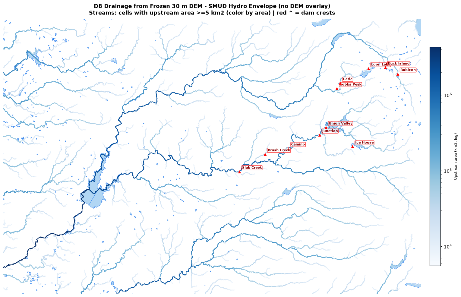
Reading the map: the dominant stem is the Feather River system draining from the high country (right/upper area, highest Strahler order ~10) down to the valley floor at lower left, with the American River and its tributaries joining in. The color scale is the upstream catchment area at each stream cell on a log scale — that is what makes the map readable. On a linear scale the main stem (thousands of km²) would paint the whole network dark blue and every side stream would be invisible. On the log scale, each order of magnitude of catchment is a visible step in color, so you can see the hierarchy of the network: the smallest mapped streams (~5 km²) in the palest blue, stepping up through the mid-size tributaries, to the dark-blue main stems. That hierarchy is the whole point of the map — it shows where water is collecting, which is the input the catchment step in Part 2 needs.

What's next

Part 2: finding the right inlet and outlet points for each plant and computing the actual catchment area — the land whose water ends up in that plant. Then the energy math: energy per m³ of water at each plant (head × turbine efficiency), translating precipitation and SWE into volume through the plant, converting IDSS forecast gridpoints into total water, and the hypsometric curve for each catchment (how snowpack readings at different elevations sum to a total). The last post ties it all together: a rough estimate of the dollar value at CAISO NP-15 block-contract pricing, with the caveats that keep it honest (minimum flows, capacity-bypassed dams, real-time price vs. block contract, and the extra value of ancillary services).